Contour lines


Introduction
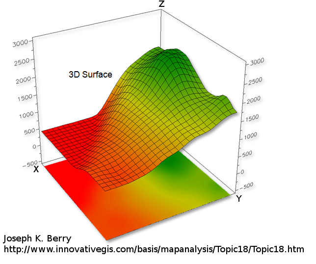
To represent a 2D function \( z = f(x,y) \) one can draw a 3D surface. The higher the \(z\) value the higher the point on the surface (see above).
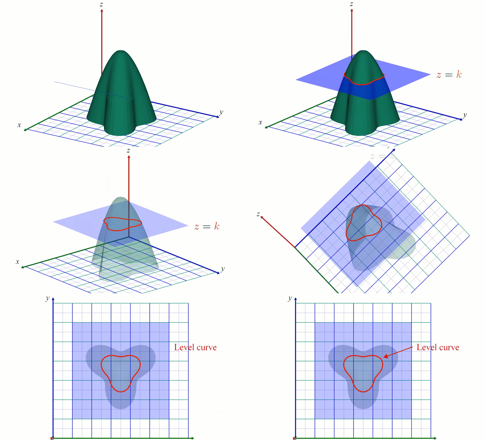
But 3D display is not always relevant, especially when used with 2D medium like paper. This is why Contour lines (sometime named level curves) are often used to display 2D functions on a flat image plane. For instance geographic maps often use level curves to display the elevation. In a map \( z \) is the terrain elevation and \((x,y)\) your location. Every points which belong to the same curve have the same height, i.e the same \( z \):

Reading contour lines
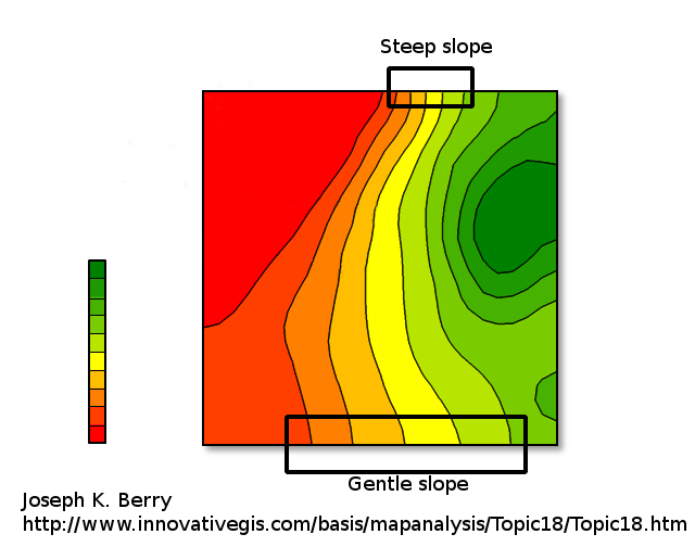
The density of the contour lines tells how steep is the slope of the terrain/function variation. When very close together it means \( f \) is varying rapidly (the elevation increase or decrease rapidly). When the curves are far from each other the variation is slower:

Gradient
One can compute the gradient of \( f \) which is a 2D vector where its two components are the partial derivative in \( x \) and \( y\) direction:
$$ \nabla f(x,y) = \begin{bmatrix} \frac{\partial f(x,y) }{ \partial x} \\ \frac{\partial f(x,y) }{ \partial y} \end{bmatrix} = \begin{bmatrix} f_x(x,y) \\ f_y(x,y) \end{bmatrix} $$
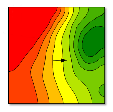
This means we measure the slope of \( f \) in \( x \) and \( y \) direction. Therefore the gradient vector \( \nabla f \) tells the direction the function varies the most. Here we show the gradient vector computed at some position and show it on the plot of \( f \) with contour lines:

The gradient is always orthogonal to the level curves. It makes sens because the gradient's direction define the steepest ascent whereas when moving along the level curve there is no slope/no variation of \( f \).
Supplement
Level curve animation (5mn43 - 7mn43)
No comments
 Donate